• Question 1
  • Preliminary Work
  • a. what could be going wrong with our calculation and a better way to evaluate this data
    • Outlier Detection
    • Distribution of Order Amount and Total Items
  • b. What metric would you report for this dataset?
    • AOV and Its Discontents
    • Improving AOV
  • c. What is its value?
  • Conclusion
• Question 2
  • a. How many orders were shipped by Speedy Express in total?
  • b. What is the last name of the employee with the most orders?
  • c. What product was ordered most by customers in Germany?

Question 1

Preliminary Work

Problem Statement: Sneakers are a relatively cheap item, given that these shops are selling sneakers, something seems to be wrong in our analysis. Our objective is to figure out (1) what could be skewing the AOV and how we can better evaluate this data (2)a better metric to report for thsi dataset (3) the value of the matric

What we know about this dataset:

• There are 100 sneaker stores in this data
• each of these shops only sells one kind of sneaker
• average order value (AOV) is $3145.13

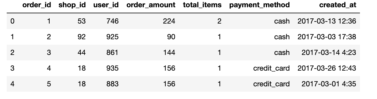
  data = pd.read_csv('sneaker_data.csv')
  data.head()
  

data-challenge

data.shape

(5000, 7)

print(data['created_at'].min())
print(data['created_at'].max())

2017-03-01 0:08
2017-03-30 9:55

Verify that our data contains no missing values:

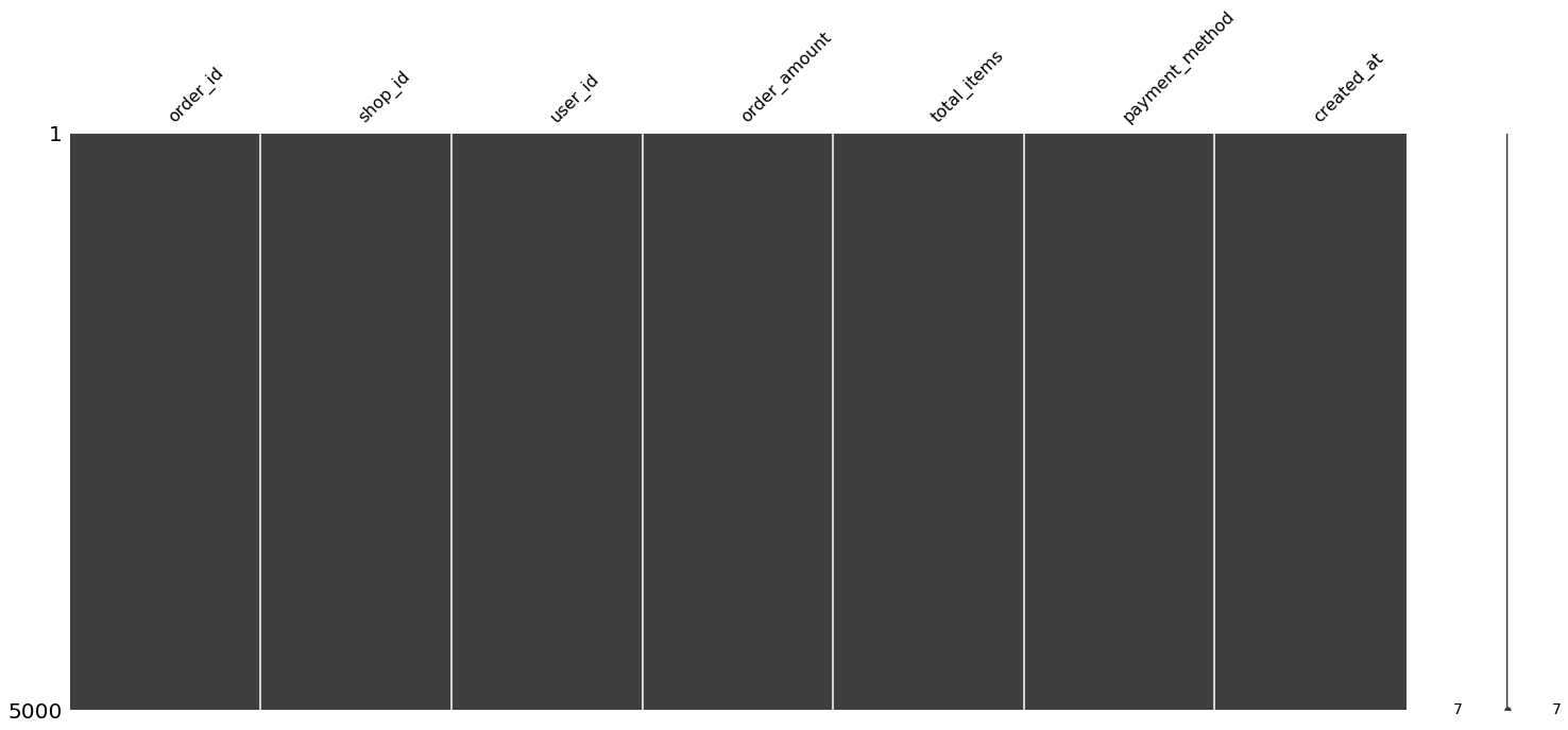
msno.matrix(data)

data.isnull().sum()

order_id          0
shop_id           0
user_id           0
order_amount      0
total_items       0
payment_method    0
created_at        0
dtype: int64

• The missing value matrix allows us to visually see if the missing values in the dataset follow any pattern.

• There are no missing values in this dataset.

a. what could be going wrong with our calculation and a better way to evaluate this data

Investigating the Flaw of Averages

# counts the number of unique shops in our data
print("Numbers of unique shops: "+ str(len(data.shop_id.unique())))

# calculate summary statistics of order_amount column
data.order_amount.describe()

Numbers of unique shops: 100

count      5000.000000
mean       3145.128000
std       41282.539349
min          90.000000
25%         163.000000
50%         284.000000
75%         390.000000
max      704000.000000
Name: order_amount, dtype: float64

Therefore, we can verify that:

• There are 100 unique stores in this dataset
• and the AOV is indeed 3145.13 dollars

However! Looking at the summary statistics of order_amount column raises red flags

• The Standard Deviation (SD) of AOV is 41,282.54 dollars, which is very large relative to the mean
• The median order value is 284 dollars while the max order value in our data set is $704,000 dollars!

This tells us us that the order amounts are spread out over an extremely wide range since the SD is 41,282.54 and although, 50% of the orders are below 284 dollars (and 75% orders are below 390.00)

Based on these facts, we have evidence which indicates our data may contain outliers..

Outlier Detection

fig = px.scatter(data, x="created_at",
                 y="order_amount", 
                 color="shop_id",log_x=False, 
                 size_max=60, template="plotly_dark",
                 hover_data=["payment_method", "total_items"],
                  labels={
                     "created_at": "Time",
                     "order_amount": "Order Amount (Dollars)",
                 },
                 title="Distribution of Sales" )

Immediately we can make note of several things about the data:

• There are two stores in particular which seem to be skewing the distribution of order_amount: shop_id =42 and shop_id = 78
• shop_id =42 has several orders where the order amount is exactly 740,000 dollars
  • however, the total_items is exactly 2000 in these orders
• data generated by shop_id =78 (orange obs.) also needs to be more carefully analyzed:
  • this shop also seems to have relatively high order_amount, compared to the rest of the orders
  • however unlike shop_id = 42, the order total_item are in the range of anywhere from 1-3 (need to verify this more rigorously)

# shop id 42
df_shop_42 = data[data['shop_id'] == 42]
fig = px.scatter(df_shop_42, x="created_at",
                 y="order_amount", 
                 color="shop_id",log_x=False, 
                 size_max=60, template="plotly_dark",
                 hover_data=["payment_method", "total_items"],
                 labels={
                     "created_at": "Time",
                     "order_amount": "Order Amount (Dollars)",
                 },
                 title="Shop ID: 42 Distribution of Sales" )
fig.show()

# shop id 78
df_shop_78 = data[data['shop_id'] == 78]
fig = px.scatter(df_shop_78, x="created_at",
                 y="order_amount", 
                 color="shop_id",log_x=False, 
                 size_max=60, template="plotly_dark",
                 hover_data=["payment_method", "total_items"],
                 labels={
                     "created_at": "Time",
                     "order_amount": "Order Amount (Dollars)",
                 },
                 title="Shop ID: 78 Distribution of Sales" )
fig.show()

Great.. but what do the above plots tell us?

They two plots above give us two important missing details of the story:

1. Shop ID: 42 seems to have sold shoes in order sizes ranging from 1-3, however, it also regularly sold shoes in bulk orders containing 2000 shoes, which bring up the order values to 704,000 dollars

2. Shop ID: 78 just sells very expensive sneakers (25,725 dollars/pair)

Therefore, we can rule out the possibility that these extreme values were generated by an imputation error or some sort of mistake.

Distribution of Order Amount and Total Items

It would be useful to see what proportion of the revenue in order_value is generated by orders where 2000 shoes were sold. Furthermore, it would also be helpful to know what the distribution of total_orders is, i.e., in what percentage orders one sneaker is purchased versus in percent of orders 2000 sneakers are ordered.

It would be useful to see order_value categorically separated into distinct bins based on the total items in the order. For example, it would be helpful to know what proportion of the revenue in order_value is generated by orders where 2000 shoes were sold. Furthermore, it would also be helpful to know what the distribution of total_orders.

A little Data Wrangling

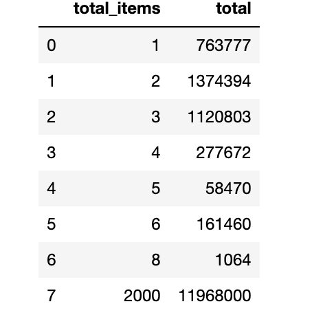
groupbyTotal = data.groupby('total_items')['order_amount'].sum().rename_axis('total_items').reset_index(name='total')
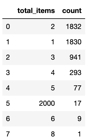
total_items_count = data.total_items.value_counts().rename_axis('total_items').reset_index(name='count')

groupbyTotal

total_items_count

We need reformat the total_items_count dataframe so the labels in both dataframes above are aligned otherwise the plot labels will not match

# aligning the dataframe labels
total_items_count  = {'total_items': 
        [1,2,3,4,5,6,8,2000],
        'count': 
        [1830,1832,941,293,77,9,1,17],
        }
total_items_count  = pd.DataFrame(total_items_count , columns = ['total_items', 'count'])

labels = [1,2,3,4,5,6,8,2000]
# Create subplots: use 'domain' type for Pie subplot
fig = make_subplots(rows=1, cols=2, specs=[[{'type':'domain'}, {'type':'domain'}]])

fig.add_trace(go.Pie(labels=labels, values=groupbyTotal['total'], name="Total Order Amounts"),
              1, 1)
fig.add_trace(go.Pie(labels=labels, values=total_items_count ['count'], name="Count"),
              1, 2)

# Use `hole` to create a donut-like pie chart
fig.update_traces(hole=.4, hoverinfo="label+percent+name")

fig.update_layout(
    title_text="Distribution of Order Amount and Total Items from 2017-03-01 to 2017-03-30",
    # Add annotations in the center of the donut pies.
    annotations=[dict(text='Total Order Amounts', x=0.145, y=0.5, font_size=12, showarrow=False),
                 dict(text='Number of Items in Order', x=0.95, y=0, font_size=16, showarrow=False)],template="plotly_dark")
fig.show()

Okay.. but what do the above plot exactly indicate? In the above figure, the first plot indicates the proportion of total order amount when we group by the total_items. So we can see that the orders from store id: 42 where 2000 total shoes were purchased, account for 76.1% ($11,968,000) of the total order amount in our dataset.

However, in the second plot, we can see that orders where 2000 shoes were purchased only make up 0.34%(17/5000) of the total order in our dataset. Therefore, these relatively few observations generated by store ID: 42 massively skew the distribution order_amount.

b. What metric would you report for this dataset?

AOV and Its Discontents

Before we jump headfirst into calculating a better metric, it might be a good idea to brainstorm advantages and disadvantages of AOV.

Since AOV is a measure of central tendency, its only a good metric if the underlying distribution is not skewed. Since total items in the orders can range anywhere from 1 to 2000, grouping them together is not an effective strategy since it results in an AOV of 3145.128000 and standard deviation of 41282.54.

Furthermore, AOV also varies widely depending on different types of sneaker stores. For instance a highend sneaker stores selling premium products (such as Shop ID: 78) will tend to have a high AOV. On the other hand, a discount store selling low priced sneaker will tend to have a low AOV.

In addition to that, the issue with using AOV is that it does not take into to account the velocity of the orders. Having a high AOV might not help you as much if the bulk of your customers are one time buyers only.

There are other long term factors which can also potentially skew the AOV if data spans a larger time frame. If most of the shoe sales occur over the holidays, the overall AOV may be much higher than what the merchant experiences in off-season times.

Improving AOV

A good metric should measure and report what is important to either the merchants, or Shopify (to improve the merachants experience selling).

So the question we should ask is: what metrics might be Shopify interested in? What metrics is the merchant interested?

No single number (metric or statistic) can capture the complexity of a distribution entirely. In many cases, looking at a single metric in isolation can be misleading. It may do more harm than good. In my experience, viewing a metric in a broader context with reference to other metrics is more insightful.

There are two main problems which skew the distribution of order_amount:

Problem (1):

• total_items ranges anywhere from orders of one sneaker to two-thousand sneakers

Solution:

• We can categorically separate orders into distinct bins based on the total items in the order before calculating AOV.

Problem (2):

• High end sneaker shops such as Shop Id: 78 will still skew the distribution of order_amounts

Solution:

• looking the standard deviation of the AOV along with the AOV gives us a better estimate of the variation of the order values.

• additionally, Median Order Value (MOV) could also be insightful when our data is skewed

c. What is its value?

Calculating the Improved Metrics

def metrics_calculator(df):
    """
    A simple function  calculates the AOV, Standard Deviation of AOV and Median Order Value

    Parameters
    ----------
    Pandas Dataframe with column 'total_items' and 'order_amount'
    
    Returns
    -------
    Pandas DataFrame
    """
    
    #calculate the AOV
    groupbyTotalItems = df.groupby('total_items')['order_amount'].mean().rename_axis('Total Items in Order').reset_index(name='AOV')
    
    # next we calculate the SD for AOV
    SD = df.groupby('total_items')['order_amount'].std().rename_axis('Total Items in Order').reset_index(name='std')['std']
    
    # calculate the Median Order Value
    median =  df.groupby('total_items')['order_amount'].median().rename_axis('Total Items in Order').reset_index(name='Median')['Median']
    
    #adding the SD and Median Order Value column to the dataframe
    groupbyTotalItems['Median Order Value'] = median
    groupbyTotalItems['Standard Deviation'] = SD
    
    return groupbyTotalItems

metrics_calculator(data)

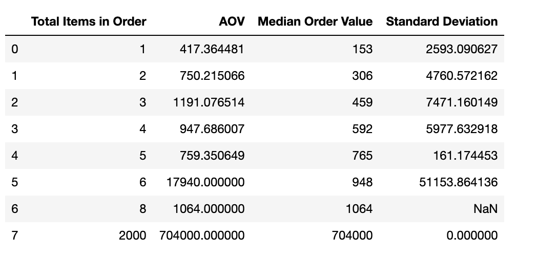
• There is only one order in the dataset where 8 items were ordered, which explains the NaN Standard deviation.
• all orders where 2000 items were ordered were valued at 704,000 which explains the 0 Standard Deviation

Conclusion

Grouping the orders based on total items in order seems to give us more reasonable AOVs. However, the standard deviation is still relatively high. There is massive variation in order amounts, even when controlled for total items in the order.

The Median Order Value (MOV) gives us additional information about the distribution of order_amounts. The MOV tells us that 50% of the orders amounts were above the median, and 50% were below. However, the median can be a tricky metric when viewed in isolation. An increase in the median order value does not indicate whether or not sales went overall. Median is just the middle value of a set of numbers. Rather than tunnel visioning on a single metric, viewing at the AOV, MOV, and the SD in combination leads to a richer understanding of the distribution of order_amounts. The gap between the MOV and AOV gives a rough estimate of the skew in the data distribution. Additionally, the SD gives information about how much the order values vary. Ultimately, the improved understanding of data allows Merchants and the Shopify Team to make more informed decisions.

Question 2

a. How many orders were shipped by Speedy Express in total?

SELECT ShipperName, COUNT(Orders.ShipperID)
FROM Orders
INNER JOIN Shippers ON Orders.ShipperID = Shippers.ShipperID
GROUP BY Orders.ShipperID;

There were 54 orders shipped by Speedy Express.

b. What is the last name of the employee with the most orders?

SELECT LastName, COUNT(Orders.EmployeeID)
FROM Orders
INNER JOIN Employees ON Orders.EmployeeID = Employees.EmployeeID
GROUP BY Orders.EmployeeID
Order by COUNT(Orders.EmployeeID) Desc;

The last of of the employee with the most orders is “Peacock”.

c. What product was ordered most by customers in Germany?

There can be two possible ways to interpret this question.

If we are interested in the quantity of the product

SELECT ProductName, MAX(Quantity)
FROM(
	 SELECT Products.ProductName as ProductName, OrderDetails.Quantity
	 FROM Orders
	 INNER JOIN Customers ON Orders.CustomerID=Customers.CustomerID
	 INNER JOIN OrderDetails ON Orders.OrderID=OrderDetails.OrderID
	 INNER JOIN Products ON Products.ProductID=OrderDetails.ProductID
	 WHERE Country = 'Germany'
	 Group By Products.ProductID
	 Order by  OrderDetails.Quantity Desc);

Steeleye Stout was purchased 100 times, was the most ordered item in Germany.

However, if we are not interested in the quantity of the product, but simply care about which product was ordered most frequently by customers, we can using the following SQL Query:

SELECT ProductName, MAX(ProductCount)
FROM (
	  SELECT Products.ProductName as ProductName, COUNT(Products.ProductName) as ProductCount
	  FROM Orders
	  INNER JOIN Customers ON Orders.CustomerID=Customers.CustomerID
	  INNER JOIN OrderDetails ON Orders.OrderID=OrderDetails.OrderID
	  INNER JOIN Products ON Products.ProductID=OrderDetails.ProductID
	  WHERE Country = 'Germany'
	  GROUP BY Products.ProductName
	  Order by COUNT(Products.ProductName) Desc
      );

Gorgonzola Telino was ordered five times, making it the most ordered product in Germany.